Deer Browse Data Exploration

In 2022, FEMC began its work compiling information related to the impacts of deer browse across the region. As a part of this effort, staff hoped to use our Forest Health Monitoring (FHM) plots to study regeneration more closely, selecting a subset of plots that were high, low, and moderately impacted by browse.

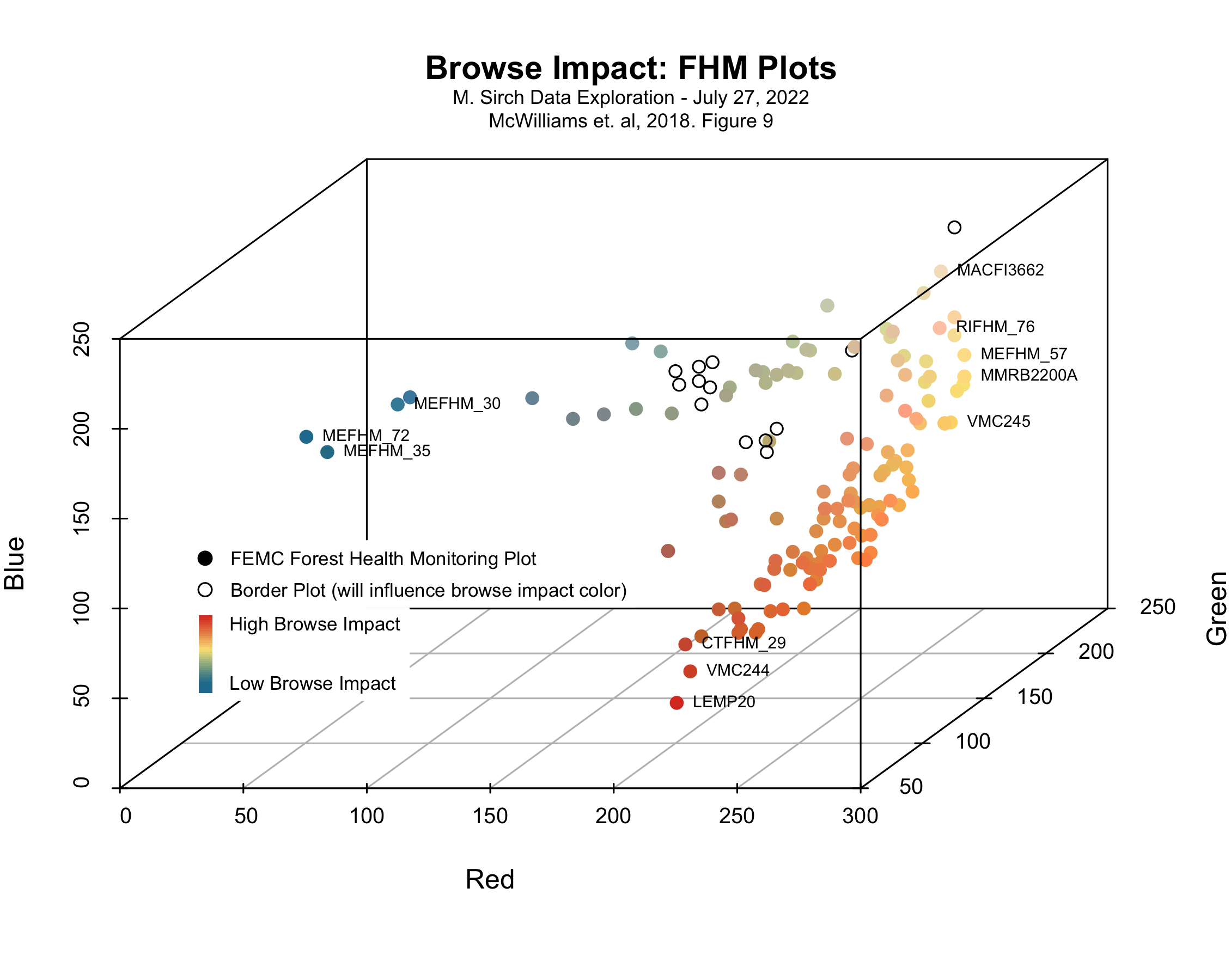
I thought it might be a fun exercise to reverse engineer browse impact data from RGB values of figure 9 of McWilliams et. al, 2018 (https://doi.org/10.2737/NRS-GTR-182). Rather than browse impact displayed in a linear continuum between red and blue, the 3D plots reveal the relationship of the browse impact and FHM plots along the red-yellow-blue gradient. We ultimately selected plots with high red maple seedling counts, but let’s reach out to the authors anyway to see what they might have to say.

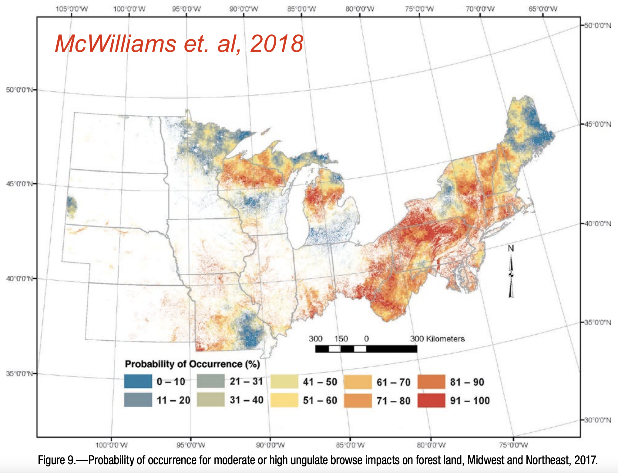
McWilliams, William H.; Westfall, James A.; Brose, Patrick H.; Dey, Daniel C.; D'Amato, Anthony W.; Dickinson, Yvette L.; Fajvan, Mary Ann; Kenefic, Laura S.; Kern, Christel C.; Laustsen, Kenneth M.; Lehman, Shawn L.; Morin, Randall S.; Ristau, Todd E.; Royo, Alejandro A.; Stoltman, Andrew M.; Stout, Susan L. 2018. Subcontinental-scale patterns of large-ungulate herbivory and synoptic review of restoration management implications for midwestern and northeastern forests. Gen. Tech. Rep. NRS-182. Newtown Square, PA: U.S. Department of Agriculture, Forest Service, Northern Research Station. 24 p. https://doi.org/10.2737/NRS-GTR-182.

Georeferencing (one of my favorite tools!)

 R Code: Static Scatterplot

## BROWSE STATIC (scatterplot3d) ##

# Code adapted by Matthias Sirch, 6/27/2022

# McWilliams et. al. 2018 (https://doi.org/10.2737/NRS-GTR-182)

install.packages("scatterplot3d")

library(scatterplot3d)

setwd("/Users/matthiassirch/Desktop/BrowseFolder")

Browse<-read.csv("Browse.csv",sep=",")

# Convert RGB value (0-256) to 0-1 range

# Display as black (rgb(0,0,0)) if color might be influenced by state border

Browse$r1<-ifelse(Browse$Border==1,0,Browse$Red/256)

Browse$g1<-ifelse(Browse$Border==1,0,Browse$Green/256)

Browse$b1<-ifelse(Browse$Border==1,0,Browse$Blue/256)

# hollow symbol for border plots

Browse$pch<-ifelse(Browse$Border==1,1,19)

# labels you want on the plot

Labels <- data.frame(PlotID = c("MACFI3662","MEFHM_72","MEFHM_35","MEFHM_30","LEMP20","VMC245","VMC244","RIFHM_76","CTFHM_29","MEFHM_57","MMRB2200A"), Label = 1, stringsAsFactors=FALSE)

Browse<-merge(Browse,Labels,by="PlotID",all=T)

Browse$Label <- replace(Browse$Label,is.na(Browse$Label),0)

# legend color ramp

# red: rgb(0.8593750,0.2382812,0.1640625)

# yellow: rgb(0.9843750,0.8945312,0.5273438)

# blue: rgb(0.1523438,0.4804688,0.6210938)

plot.new()

lgd_ = rep(NA, 60)

lgd_[c(2,58)] = c("High Browse Impact","Low Browse Impact")

legend(x = .78, y = 1,

legend = lgd_, fill = colorRampPalette(colors = c(rgb(0.8593750,0.2382812,0.1640625),rgb(0.9843750,0.8945312,0.5273438),rgb(0.1523438,0.4804688,0.6210938)))(60),

border = NA,

y.intersp = .1,

cex = .7, text.font = 1)

##################################################################

# EXPORT #########################################################

##################################################################

# Perspective for plot output

degrees<-45

###########

# to export frames for video/gif

# run code within loop to export single frame

# image set for 45 degrees

for (degrees in 1:360){

graphics.off()

png(filename = paste0("Browse",degrees,".png"), width = 8, height = 6, units = "in", res = 300)

par(mai = c(0.5, 0.5, 0.5, 0.5))

BrowsePlot<-scatterplot3d(x = Browse$Red, y = Browse$Green, z = Browse$Blue,main="Browse Impact: FHM Plots",

mtext("M. Sirch Data Exploration - July 27, 2022\nMcWilliams et. al, 2018. Figure 9", side = 3, cex=.72),

xlab = "Red", ylab = "Green", zlab = "Blue",

color = rgb(Browse$r1,Browse$g1,Browse$b1,1),

cex.symbols = 1, pch = Browse$pch, angle = degrees,grid = TRUE)

lgd_ = rep(NA,30)

lgd_[c(2,28)] = c("High Browse Impact","Low Browse Impact")

legend(x = .5, y = 2,

legend = lgd_,

fill = colorRampPalette(colors = c(rgb(0.8593750,0.2382812,0.1640625),rgb(0.9843750,0.8945312,0.5273438),rgb(0.1523438,0.4804688,0.6210938)))(30),

border = NA,bty='y',

y.intersp = .1,

cex = .7, text.font = 1,box.col = "white")

lgd_FHM="FEMC Forest Health Monitoring Plot"

legend(x = 0.44, y =2.75,

legend = lgd_FHM,

pch=19, pt.cex=1.1,

y.intersp = .5, x.intersp = 1.49,

fill = "white",

border = NA,bty='y',

cex = .7, text.font = 1, box.col = "white")

lgd_Border="Border Plot (will influence browse impact color)"

legend(x = 0.44, y =2.4,

legend = lgd_Border,

pch=1, pt.cex=1.1,

y.intersp =.5, x.intersp = 1.49,

fill = "white",

border = NA,bty='y',

cex = .7, text.font = 1, box.col = "white")

BrowsePlot.coords <- BrowsePlot$xyz.convert(Browse$Red,Browse$Green,Browse$Blue)

text(BrowsePlot.coords$x,

BrowsePlot.coords$y,

labels = ifelse(Browse$Label=="1",as.character(Browse$PlotID),""),

cex = .6,

pos = 4)

dev.off()

}

  R Code: Interactive Scatterplots

## BROWSE INTERACTIVE (plotly) ##

# Code adapted by Matthias Sirch, 6/27/2022

# McWilliams et. al. 2018 (https://doi.org/10.2737/NRS-GTR-182)

install.packages("plotly")

library(plotly)

setwd("/Users/matthiassirch/Desktop/BrowseFolder")

Browse<-read.csv("Browse.csv",sep=",")

# Convert RGB value (0-256) to 0-1 range

# Display as black (rgb(0,0,0)) if color might be influenced by state border

Browse$r1<-ifelse(Browse$Border==1,0,Browse$Red/256)

Browse$g1<-ifelse(Browse$Border==1,0,Browse$Green/256)

Browse$b1<-ifelse(Browse$Border==1,0,Browse$Blue/256)

# hollow symbol for border plots

Browse$pch<-ifelse(Browse$Border==1,1,19)

BrowseInteractive <- plot_ly(Browse, x = ~Red, y = ~Green, z = ~Blue,

text = ~PlotID,

hoverinfo = "text",

mode = 'markers', symbol = Browse$pch, symbols = c('o','circle'),

marker = list(color = rgb(Browse$r1,Browse$g1,Browse$b1,1)))

BrowseInteractive

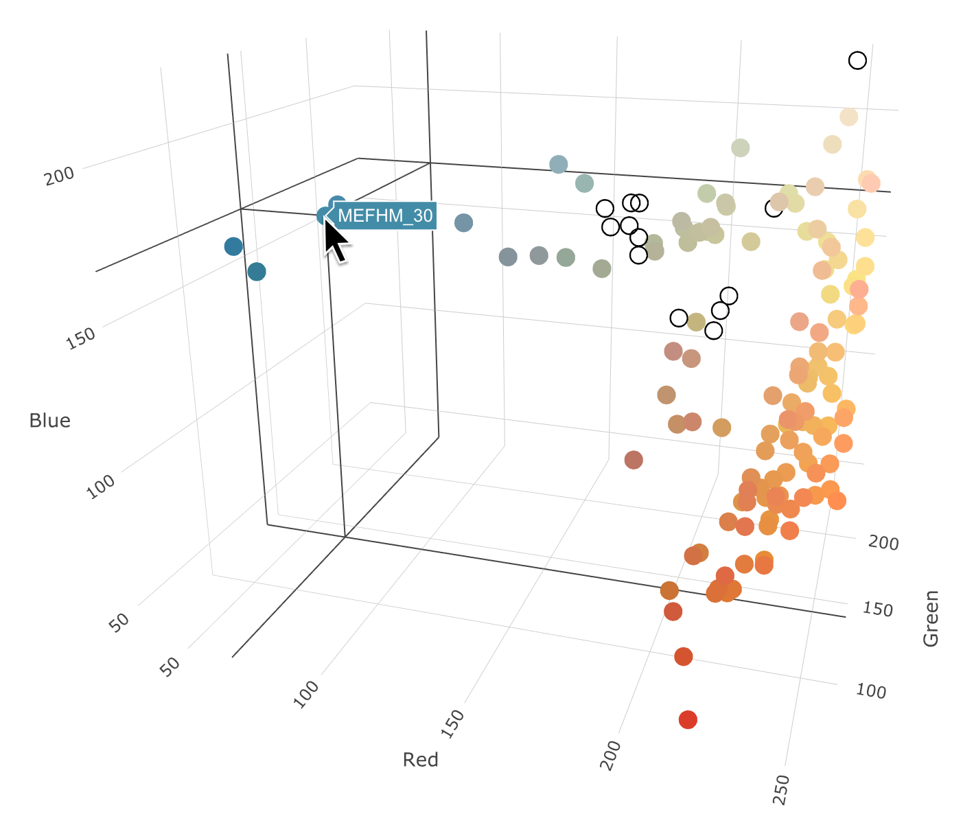
Plot is not interactive here, but these are neat - you should try it!